TL;DR
We discover that attention head representations in vision transformers lie on low-dimensional manifolds where principal components encode specialized semantics (letters, locations, animals, etc.).
By selectively amplifying task-relevant principal components through learned anisotropic scaling (ResiDual), we achieve fine-tuning level performance with up to 4 orders of magnitude fewer parameters than full fine-tuning.
8.3k-14k
Learnable parameters
(vs. 300M for full fine-tuning)
0.90-0.92
Average accuracy
(matching full fine-tuning)
0.97
Cross-model correlation
(universal spectral structure)
Overview
When examined through the lens of their residual streams, a puzzling property emerges in transformer networks: residual contributions (e.g., attention heads) sometimes specialize in specific tasks or input attributes. ResiDual reveals that this specialization is encoded in the principal components of attention head representations—and that this structure can be exploited for highly parameter-efficient fine-tuning.
Much like panning for gold, ResiDual selectively amplifies task-relevant principal components while dampening noise from irrelevant attributes. By operating at the spectral level, it achieves fine-tuning level performance with up to 4 orders of magnitude fewer parameters than full fine-tuning, and 2 orders less than training a simple linear transformation at the output.
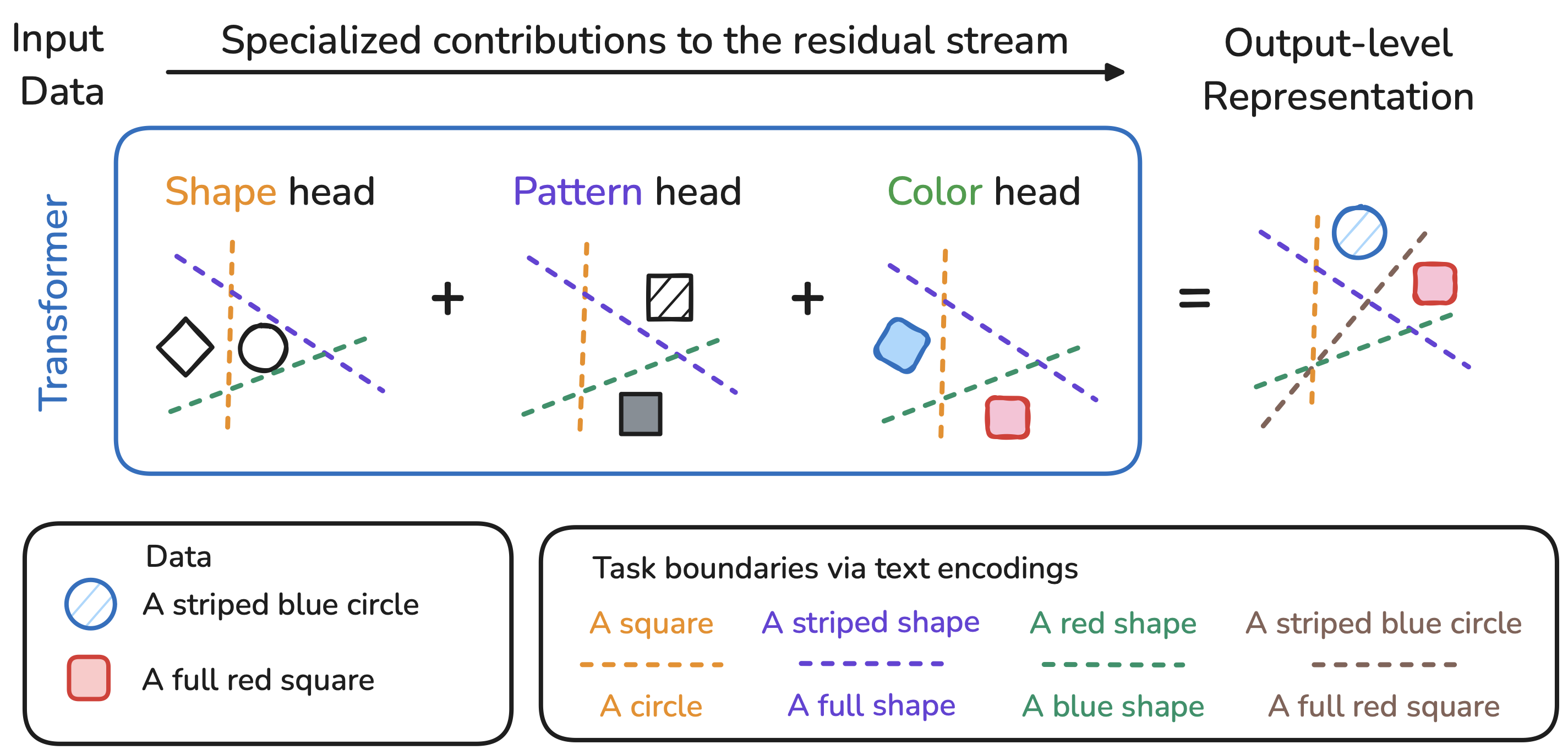
Method: Spectral Geometry of Residual Units
Low-Dimensional Structure of Attention Heads
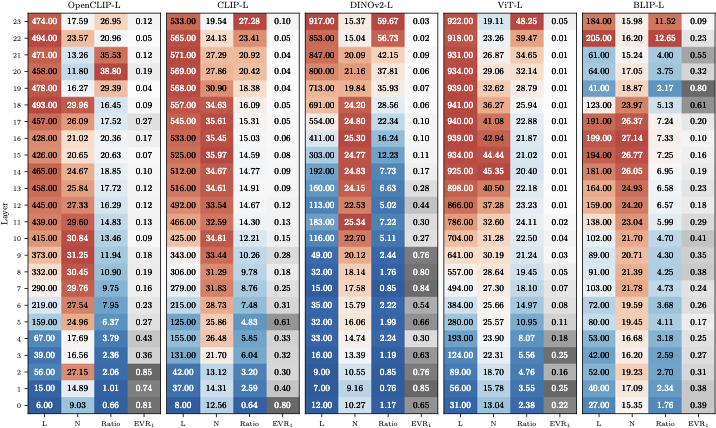
Our analysis begins with a fundamental observation: despite being embedded in high-dimensional spaces, attention head representations lie on low-dimensional manifolds. We measure this using both linear (PCA) and nonlinear (TwoNN) intrinsic dimensionality estimators across multiple vision transformer architectures.
Intrinsic Dimensionality Analysis
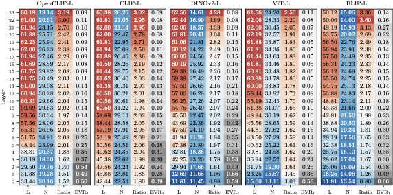
Analysis across ViT-Large architectures showing:
- L Linear dimensionality from PCA
- N Nonlinear dimensionality from TwoNN
- Ratio L/N indicating nonlinearity
- EVR₁ First principal component variance
Key findings:
- Early layers: Heads are highly linear (L≈N) and low-dimensional, with the first principal component explaining ~50% of variance
- Mid-to-late layers: True dimensionality (N) follows a characteristic “hunchback” shape, peaking mid-network then decreasing
- Increasing nonlinearity: The L/N ratio grows steadily, indicating heads in deeper layers lie on curved manifolds
- Persistent structure: Even in the deepest layers, the first PC still explains ~10% of variance
- Universal pattern: This holds across different architectures (CLIP, BLIP, DINOv2, ViT) and training objectives (supervised, self-supervised, contrastive)
Principal Components Encode Specialized Semantics
We establish a crucial connection between sparse recovery methods (TextSpan) and principal component analysis. By comparing TextSpan (which operates on full head representations) with Orthogonal Matching Pursuit (OMP) applied to the first principal component alone, we find that for many specialized heads, the first PC captures nearly all semantic information.


Example specialized heads:
- L22.H8 (Letters): Z=4.93 - Nearly perfect agreement; first PC encodes letter detection
- L21.H11 (Location): Z=2.73 - Strong agreement on geographic locations
- L23.H2 (Animals): Z=1.91 - Moderate agreement on animal categories
- L20.H8 (Scenery): Z=0.02 - Low agreement; specialization distributed across multiple PCs
Cross-Dataset Spectral Analysis
Spectral Similarity Reveals Semantic Structure
We introduce a Spectral Cosine Similarity metric that compares the principal component bases of head representations across different datasets. This reveals which heads specialize for particular data distributions.
Cross-Dataset Spectral Similarity Heatmap
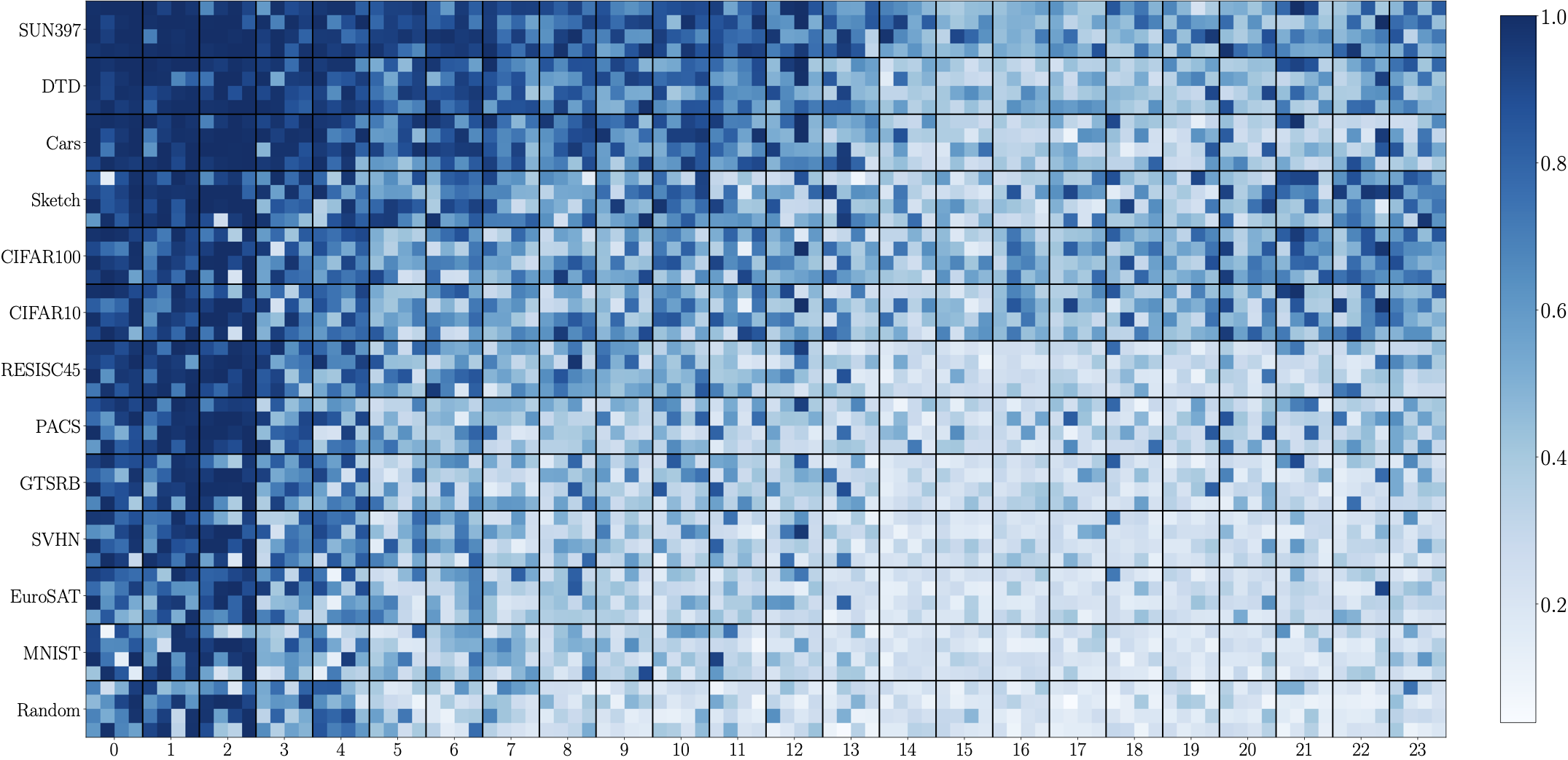
Early Layers (L0-L10):
Nearly uniform high similarity across all datasets → universal low-level features
Late Layers (L18-L23):
Sparse, dataset-specific patterns → specialized semantic heads
Key observations:
- Universal low-level features: Early layers (L0-L10) show nearly uniform high similarity across all datasets, including random noise
- Emergent specialization: Late layers (L18-L23) show sparse patterns where specific heads activate only for semantically relevant datasets
- Semantic coherence: Heads specialize predictably:
- L22.H7 (Seasons): High similarity for outdoor scenery datasets (EuroSAT, GTSRB, SUN397)
- L22.H11 (Grayscale): Low similarity for ImageNet-Sketch (grayscale drawings)
- L23.H10 (Numbers): High similarity for MNIST and SVHN (digit datasets)
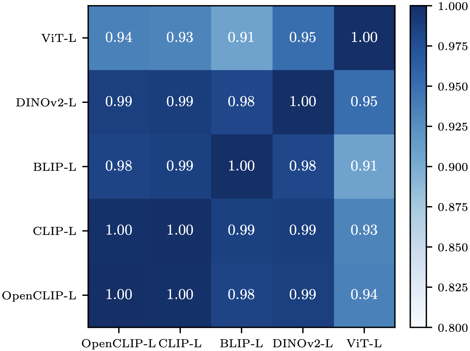
- Cross-model consistency: Dataset similarity rankings show 0.97 Pearson correlation across different models (CLIP, BLIP, DINOv2, ViT)—indicating architectural invariance
Universal Spectral Structure Across Architectures
The spectral specialization patterns we observe are remarkably consistent across different model architectures, training objectives, and pretraining data. This universality suggests that the geometric structure of attention head representations reflects fundamental properties of visual features.
Transformer Alignment Experiments
Zero-Shot Classification via Head Selection
Before introducing spectral reweighting, we first ask: Are all heads necessary for a given task? We evaluate several strategies for selecting the top 5% of heads:
- Unsupervised (U): Head-to-output correlation
- Task-conditioned (U|T): Correlation conditioned on task subspace (CompAttribute)
- Supervised (S): Direct task performance evaluation (logit lens)
- Random (R): Random selection baseline
- Optimized (O): Continuous weights via gradient descent (upper bound)
| Configuration | BLIP-L | OpenCLIP-L |
|---|---|---|
| Random (R) | 0.28 | 0.33 |
| All Heads (H) | 0.53 | 0.62 |
| Unsupervised (U) | 0.58 | 0.71 |
| Supervised (S) | 0.61 | 0.73 |
| Base Model (B) | 0.59 | 0.70 |
| Optimized (O) | 0.76 | 0.84 |
Key insights:
- Heads dominate: Attention heads alone (H) provide ~90% of the performance (comparing H to B)
- Sparse sufficiency: Top 5% of heads match or exceed full model performance
- Unsupervised effectiveness: Simple correlation with output works surprisingly well
- Hidden potential: Continuous optimization (O) can nearly double performance on some datasets (e.g., SVHN: 0.33→0.81), revealing that task-relevant information already exists but is obscured
Semantic Coherence of Selected Heads
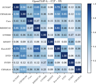
When we examine which heads are selected across different datasets, we find that semantically similar tasks consistently select overlapping sets of heads. This validates that head specialization is stable and transferable across related domains.
ResiDual: Spectral Anisotropic Scaling
Rather than selecting entire heads, ResiDual operates at the finer granularity of principal components within each head. This allows for more nuanced control over which semantic features to amplify or dampen.
Method Formulation
Given head representation $$\mathbf{X}$$, PCA basis $$\mathbf{\Phi}$$, and mean $$\mathbf{\mu}$$:
where $$\mathbf{\lambda}$$ is a learnable vector of weights for each principal component. The full residual stream is transformed as:
- RD All PCs of all residual units (heads + MLPs)
- RD* Heads only, PCs truncated to 90% variance (parameter-efficient)
- RD^Y ResiDual applied directly to output encoding
- Lin Linear transformation at output level
- Full FT Finetune entire ViT with frozen text encoder

Diamond plot showing accuracy across 10 datasets for BLIP-L, CLIP-L, and OpenCLIP-L. RD* (heads-only, 90% variance) closely tracks Full Finetuning while using orders of magnitude fewer parameters. SVHN shows the largest gap between Base and ResiDual (~0.2-0.4 improvement), indicating task features buried deep in the residual stream.
| Method | BLIP-L | CLIP-L | OpenCLIP-L | Parameters |
|---|---|---|---|---|
| Base | 0.59 | - | 0.70 | 0 |
| Lin | 0.86 | 0.89 | 0.91 | 65.8k-590k |
| RD | 0.88 | 0.90 | 0.92 | 30.7k-43k |
| RD* | 0.86 | 0.90 | 0.91 | 8.3k-14k |
| RD^Y | 0.74 | 0.82 | 0.84 | 256-768 |
| Full FT | ~0.88 | ~0.91 | ~0.93 | ~300M |
- BLIP-L: Base 0.33 → Lin 0.65 → RD 0.81 → RD* 0.77
- CLIP-L: Base 0.58 → Lin 0.77 → RD 0.86 → RD* 0.86
- OpenCLIP-L: Base 0.41 → Lin 0.75 → RD 0.86 → RD* 0.85
The large gap between RD* and RD^Y on SVHN (e.g., 0.77 vs 0.53 for BLIP-L) confirms that task-relevant features are buried in the residual stream, not accessible at the output level.
Beyond Multimodal Models
Generalization to Unimodal Encoders
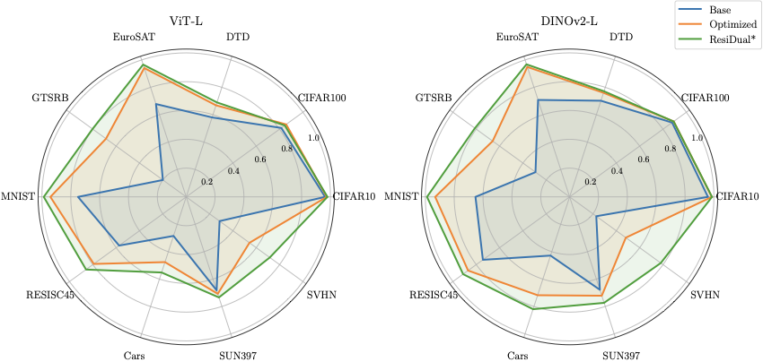
ResiDual’s spectral approach is not limited to multimodal models like CLIP. We demonstrate that the same principles apply to unimodal vision encoders (DINOv2, ViT) using prototypical classifiers, where class prototypes are computed as mean embeddings of training samples per class.
Key findings:
- Method generality: ResiDual framework applies to unimodal encoders using prototypical classifiers
- Self-supervised advantage: DINOv2-L (self-supervised) outperforms ViT-L (supervised) in this setting
- Consistent patterns: Same datasets (SVHN, GTSRB) remain challenging; same methods provide improvements
Why Focus on Attention Heads?
Our analysis reveals a crucial distinction between attention heads and MLP units: while heads exhibit low-dimensional, interpretable spectral structure with clear semantic specialization, MLPs show higher dimensionality and strong concept superposition.
Key Findings
Citation
@article{basile2025residual,
  title   = {ResiDual Transformer Alignment with Spectral Decomposition},
  author  = {Basile*, Lorenzo and Maiorca*, Valentino and
             Bortolussi, Luca and Rodol{\`a}, Emanuele and Locatello, Francesco},
  journal = {Transactions on Machine Learning Research},
  year    = {2025},
  url     = {https://openreview.net/forum?id=z37LCgSIzI}
}
Authors
Lorenzo Basile¹’² · Valentino Maiorca²’³’⁴ · Luca Bortolussi¹ · Emanuele Rodolà³ · Francesco Locatello⁴
¹University of Trieste, Italy · ²Work done while visiting ISTA · ³Sapienza University of Rome, Italy · ⁴Institute of Science and Technology Austria (ISTA)